Introduction
Then finance and banking industry has gone through massive shifts in the in the last decade. Between the downturn from the financial crisis in 2008 and the increasingly disruptive pressure from Silicon Valley it is even more important to understand our customers’ behavior. (Deloitte, 2016) Direct sales marketing is one of the most effective methods for both gaining new customers as well as increasing the deposits of our existing customers. Globalytics Capital needs to gain better insight into its customer’ behavior to be poised for success in the future. In order to position Globalytics Capital the Data Access Response Team (D.A.R.T) is proposing an analysis be done using the customer marketing database.
Analysis Method
As a proof of concept D.A.R.T. has created this report detailing how such an analysis could be conducted using a similar banking database. The data that D.A.R.T will be utilizing comes from the Center for Machine Learning and contains the result of direct marketing campaigns from another banking institution. (Moro, Cotez, & Rita, 2014) Globalytics Captial conducts similar campaigns throughout the year. A direct marketing campaign consists of phone calls made to potential customers with the positive outcome being a deposit made with the bank. The data set that we will be looking at contains 17 input attributes and one output attribute. The input attributes are organized in 3 groups.
- Bank Client Data
- Last Contact Data
- Extended Contact Data
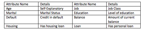
Bank Client Data
This is demographic data about the customer being contacted. The information captured here helps the marketer better understand the customer’s life circumstances and whether they have existing loans. The following table details these attributes.
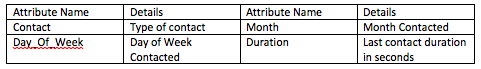
Last Contact Data
This is data about the last contact with the customer during the current campaign. It is important to know how long it has been between customer contacts. Too frequent contacts can result in negative outcomes with customers so marketers need to know this information.
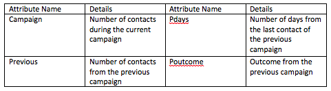
Extended Contact Data
This data gives us additional information about the current campaign as well as the previous marketing campaign. This is important to understand how this customer has responded in the past.
Finally, there is the output variable labeled y which shows whether the call was successful.
Data Mining Approach
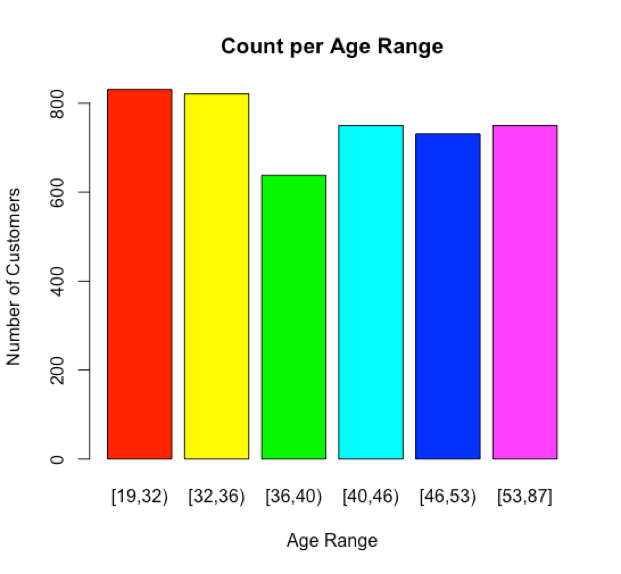
For this example, the apriori algorithm will be used to determine the which customers will be most likely to make a deposit during a marketing campaign. This will allow us to prioritize the customers during the campaign. Several of the fields within this data set will need to be modified before any processing can being. Six of the fields will need to be changed from continuous numeric fields into discrete bins. Specifically, the age, balance, duration, campaign, pdays, and previous fields need to be modified. This allows us to count the number of rows. The below chart shows the age range pins.
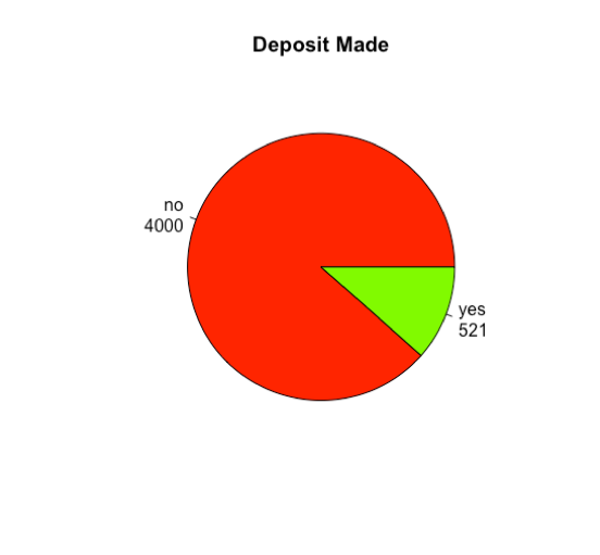
Interpretation
Within the data set there were a total of 4521 calls made during this campaign. 521 calls were successful while 4000 were not successful resulting in a 11% success rate for this campaign. This again shows the importance for knowing which customers to target.
After interpreting the data, it was determined that there were only 2 conditions that have an impact on the outcome of a solicitation call. Customers with no personal loans and nothing in default are the most likely to respond favorably. For both of these conditions the algorithm returned with around 12% confidence. This is not a high level of confidence however this is in line with the 11% success rate for the campaign.
Conclusions
Moving forward the team feels that we should adjust the bins for some of the continuous fields. This would allow for rule sets with a higher support and confidence levels. The data set was a small sample of the data that would be available from Globalytics Capital. With a larger data set there would be a greater opportunity for building association rules.
References
- Deloitte. (2016, July 1). Banking Industry Outlook: Banking reimagined. Retrieved Oct 17, 2016, from Deloitte: http://www2.deloitte.com/us/en/pages/financial-services/articles/banking-industry-outlook.html
- Moro, S., Cotez, P., & Rita, P. (2014, June 1). Bank Marketing Data Set. Retrieved from Machine Learning Repository: https://archive.ics.uci.edu/ml/datasets/Bank+Marketing
Apendix A – R Code
library(arules)
library(arulesViz)

setwd("~/Documents/DATA 630 FALL 2016/Assignment 3/bank")
bank <- read.csv("~/Documents/DATA 630 FALL 2016/Exercise 3/Bank.csv")
str(bank)
bank$age <- discretize(bank$age, "frequency", categories=6)
bank$balance <- discretize(bank$balance, "frequency", categories=6)

bank$duration <- discretize(bank$duration, "frequency", categories=6)

bank$campaign <- discretize(bank$campaign, "frequency", categories=6)

bank$pdays <- discretize(bank$pdays, "frequency", categories=6)

bank$previous <- discretize(bank$previous, "frequency", categories=6)
rules<-apriori(bank, parameter=list(supp=0.1, conf=0.1, minlen=2), appearance=list(rhs=c("y=yes"), default="lhs"))
rules.sorted <- sort(rules, by="lift")
subset.matrix <- is.subset(rules.sorted, rules.sorted)
subset.matrix[lower.tri(subset.matrix, diag=T)] <- NA

redundant <- colSums(subset.matrix, na.rm=T) >= 1

rules.pruned <- rules.sorted[!redundant]
plot(bank$age, col=rainbow(6), xlab="Age Range", ylab="Number of Customers", main="Count per Age Range")
lbls <- paste(names(table(bank$y)), "\n", table(bank$y), sep="")
pie(table(bank$y), col=rainbow(4), main="Deposit Made", labels=lbls)